REFEFO Potential to Enhance Productive Connectivity

Most countries in the region have some sort of strategy to improve digital connectivity for vulnerable populations, for those who live in low density areas where the private sector alone does not have the incentives to invest in infrastructure, or to bring connectivity to education and health services. However, we cannot say the same about productive connectivity, meaning, connectivity infrastructure oriented towards improving the productivity of companies and workers.

An important prerequisite for bringing connectivity to a place is the existance of backbone networks that allow the development of the so-called “last mile” to connect homes and businesses. Argentina, for example, has the Federal Fiber Optic Network (REFEFO) managed by ARSAT, which is a backbone network that goes through the 23 provinces of the country, reaching about 1,300 localities, many of which have populations of less than 10,000 people. Of course, there are also other backbone fiber optic networks of private operators, but the layout of these networks and the location of the connection nodes is not publicly available.

But going back to the previous point, let’s analyze the potential of REFEFO to improve productive connectivity. Let’s take for example the agricultural sector, which is one of the most important in the Argentine economy and the most important regarding exports.

We can use data from the former Ministry of Productive Development to georeference agricultural companies and calculate the distance of each of them to the nearest REFEFO node and then analyze the distribution of these distances.

First, we will obtain, filter and merge the necessary data for the analysis:

import pandas as pd
import geopandas as gpd
from requests import Request
from shapely.geometry import box

# Obtengo los datos de establecimientos productivos
estab = pd.read_csv('https://cdn.produccion.gob.ar/cdn-cep/establecimientos-productivos/distribucion_establecimientos_productivos_sexo.csv')

# Obtengo datos del nomenclador de AFIP
clae = pd.read_csv('https://cdn.produccion.gob.ar/cdn-cep/clae_agg.csv')

# Uno los datos de establecimientos con el nomenclador
estab = estab.merge(clae[['clae6', 'letra_desc']], left_on='clae6', right_on='clae6')

# Filtro los del sector agropecuario
estab_agro = estab[estab['letra_desc'] == ' AGRICULTURA, GANADERÍA, CAZA, SILVICULTURA Y PESCA']

# Transformo los datos de establecimientos a un GeoDataFrame
estab_agro_gpd = gpd.GeoDataFrame(estab_agro, geometry=gpd.points_from_xy(estab_agro.lon, estab_agro.lat), crs='EPSG:4326')

# Obtengo los datos de los nodos de REFEFO
idecom_url = 'https://www.idecom.gob.ar/geoserver/ows'
params = {
    'service': 'wfs',
    'version': '1.3.0',
    'request': 'GetFeature',
    'typeName': 'idera:a010504-NODOS-FO',
    'outputFormat': 'json'
}

refefo_nodos_url = Request('GET', idecom_url, params=params).prepare().url

refefo_nodos = gpd.read_file(refefo_nodos_url)

# Obtengo los datos de la geometría de las provincias
ign_url = 'https://wms.ign.gob.ar/geoserver/ows'
params = {
    'service': 'wfs',
    'version': '1.1.0',
    'request': 'GetFeature',
    'typeName': 'ign:provincia',
    'outputFormat': 'json'
}

prov_url = Request('GET', ign_url, params=params).prepare().url
prov = gpd.read_file(prov_url)

# Recorto las provincias a la parte continental de Argentina
bbox = (-76.36532,
        -56.75009,
        -51.20850,
        -20.91625)
bbox = gpd.GeoSeries([box(*bbox)], crs=prov.crs)

prov_clipped = gpd.clip(prov, bbox)

# Cruzo los establecimientos agropecuarios con el nodo de REFEFO más cercano y obtengo la distancia
estab_agro_refefo_gpd = estab_agro_gpd.to_crs(crs=3857).sjoin_nearest(refefo_nodos.to_crs(3857), how='left', distance_col='distance')

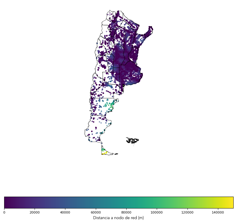
Then we will plot on a map each of the agricultural establishments and assign a color based on the distance to the nearest REFEFO node.

from matplotlib import cm
import matplotlib as mpl
import matplotlib.pyplot as plt

# Size
fig_size_bar = (7, 4)
size_labels = 10
size_tick_labels = 8

fuente_bar_pos_x = 0.0
fuente_bar_pos_y = -0.4

fuente_map_pos_x = -74.0
fuente_map_pos_y = -59.0

fontname = 'Avenir'
font_weight = 'ultralight'

norm = mpl.colors.Normalize(vmin=0, vmax=150000)

fig, ax = plt.subplots(figsize=(10, 10))

prov_clipped.boundary.plot(ax=ax, color='black', linewidth=0.5)

estab_agro_refefo_gpd.to_crs('EPSG:4326').plot(ax=ax, c=estab_agro_refefo_gpd['distance'], markersize=5, alpha=0.5, legend=True)

ax.set_axis_off()

cbar = fig.colorbar(cm.ScalarMappable(norm), ax=ax, orientation='horizontal')
cbar.set_label('Distancia a nodo de red (m)', fontname=fontname, fontsize=size_labels, weight=font_weight)
cbar.ax.tick_params(labelsize=size_tick_labels)
plt.show()

Mapa de Establecimientos Agropecuarios y Distancia a Nodo de REFEFO

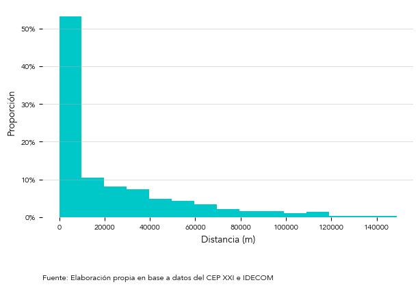
Also, we will plot the histogram of the distances to analyze their distribution.

import matplotlib.ticker as mticker
import numpy as np

color1 = [160.0/255.0, 160.0/255.0, 160.0/255.0, 1.0]
color2 = [0.0, 200.0/255.0, 200.0/255.0, 1.0]
color3 = [0.0, 255.0/255.0, 255.0/255.0, 1.0]
color4 = [94.0/255.0, 144.0/255.0, 227.0/255.0, 1.0]
color5 = [111.0/255.0, 109.0/255.0, 163.0/255.0, 1.0]

colors = [color1, color2, color3, color4, color5]

# Style
def crossval_style(ax):
    ax.spines['top'].set_visible(False)
    ax.spines['right'].set_visible(False)
    ax.spines['left'].set_visible(False)
    ax.spines['bottom'].set_visible(False)
    ax.grid(axis='y', linestyle='-', alpha=0.4)

counts, bins = np.histogram(estab_agro_refefo_gpd[estab_agro_refefo_gpd['distance'] < 150000]['distance'], bins=15)

density = counts / np.sum(counts)

fig, ax = plt.subplots(figsize=(7, 4))

# ax = estab_agro_refefo_gpd[estab_agro_refefo_gpd['distance'] < 150000]['distance'].hist(density=True, bins=15)
ax.hist(bins[:-1], bins, weights=density, color=colors[1])

# Format the yticklabels to show actual proportions
# ax.yaxis.set_major_formatter(mticker.PercentFormatter(xmax=0.0001))
ax.yaxis.set_major_formatter(mticker.PercentFormatter(xmax=1))

# Set the font family and size of the x-axis label
ax.set_xlabel('Distancia (m)', fontname=fontname, fontsize=size_labels, weight=font_weight)

# Set the font family and size of the y-axis label
ax.set_ylabel('Proporción', fontname=fontname, fontsize=size_labels, weight=font_weight)

# Set the font family and size of the x-axis tick labels
ax.set_xticklabels(ax.get_xticklabels(), fontname=fontname, fontsize=size_tick_labels, weight=font_weight)

# Set the font family and size of the y-axis tick labels
ax.set_yticklabels(ax.get_yticklabels(), fontname=fontname, fontsize=size_tick_labels, weight=font_weight)

crossval_style(ax)

ax.text(x = fuente_bar_pos_x, y = -0.3, s = f"Fuente: Elaboración propia en base a datos del CEP XXI e IDECOM", transform=ax.transAxes, fontname=fontname, fontsize=size_tick_labels, weight=font_weight)

plt.show()

Histograma de Distancias a Nodo de REFEFO

As you can see in the map and in the histogram, most of the agricultural establishments are located less than 10 km from a REFEFO node. To get the precise numbers let’s take a look at the mean and the quartiles of the distances.

estab_agro_refefo_gpd['distance'].describe()

The mean distance of agricultural establishments to the nearest REFEFO node is 25,544 meters or 25.5 KMs. However, as observed in the histogram, the distances do not have a normal distribution but rather a right-skewed distribution, with most distances having low values and a few distances having very high values. In these cases, the median is more representative than the mean. Here the median is 8,580 meters or 8.6 KMs. This means that 50% of the agricultural establishments are located less than 8.6 KMs from a REFEFO node. Finally, the third quartile is 35,895 meters or almost 36 KMs, which means that 75% of the agricultural establishments are located less than 36 KMs from a REFEFO node.

There are many ways in which we can improve this preliminary analysis but this first approach seems to indicate that the distance to backbone networks should not be an obstacle for the development of productive rural connectivity in Argentina.